---
pagetitle: "Degrees of Freedom and Robot Models of the Human Body"
description: "Admissible motion, club-task redundancy, torque and contact dynamics, physically consistent robot models, and identifiable golf experiments."
css: ../../../css/machine-learning.css
bibliography: ../golf_physics.bib
---
# Degrees of Freedom and Robot Models of the Human Body {#sec-23_dof_urdf_models}
How many independent numbers describe a golf swing? The answer depends on what the model retains. Joint angles describe configuration; velocities describe how that configuration is changing; muscle activation and elastic deformation may require additional states. Two hands gripping one club and two feet contacting the ground connect these descriptions through constraints and forces. Counting the entries in a motion-capture file does not settle any of these questions.
This chapter develops a consistent route from anatomy to computation. We first count admissible motions, then ask which of them change a declared club task, then derive how applied torques affect that task. Finally, we encode a physical mechanism and check the imported dynamics against independent mechanics. Each step answers a different question. Their connection is the foundation for interpreting a swing, designing an experiment and testing a proposed control explanation.
A rigid-body model uses the same mechanical laws for a robot and a golfer, but this does not make its joints, actuators or objectives biologically complete. Our upper-body teaching model has 20 internal freedoms before the two-hand loop is closed. That is a declared approximation, not a universal anatomical count. The executable example is a complete two-link mechanism whose limitations are explicit; extending it to a golfer requires the additional modeling decisions developed below.
[]{#computing-the-equations-of-motion-automatically}
## Counting Degrees of Freedom --- The Robotics Way
[]{#laymans-box:ch23_dof_problem}
[]{#sec-grubler_formula}
[]{#the-formula}
[]{#urdf-for-a-2-link-planar-arm}
### The Formula and Its Rank Assumption
For a spatial assembly containing $N$ bodies including one fixed reference body, begin with $6(N-1)$ unconstrained freedoms. A joint permitting $f_i$ relative freedoms nominally imposes $6-f_i$ constraints. If those constraints are independent at a regular configuration, the mobility is
$$
d=6(N-1)-\sum_{i=1}^{J}(6-f_i).
$$
[]{#thm-grubler}
This is the spatial Grübler--Kutzbach count. The independence assumption is essential. A negative result signals an inappropriate or dependent-constraint count; it is not a physical negative mobility. Special geometric arrangements and closed loops require a rank calculation. The [Modern Robotics mobility lesson](https://modernrobotics.northwestern.edu/nu-gm-book-resource/2-2-degrees-of-freedom-of-a-robot/) illustrates precisely this limitation.
With generalized velocities $v\in\mathbb R^{n_v}$ before additional closures, let $A(q)v=0$ describe independent, stationary constraints. At a regular configuration,
$$
d=n_v-\operatorname{rank}A(q).
$$
For holonomic constraints $\phi(q)=0$ in local coordinates with $\dot q=v$, $A=D\phi$. With quaternion coordinates, $\dot q=E(q)v$ and $A=D\phi\,E$. Do not subtract the quaternion normalization constraint a second time from $n_v$: it has already been accounted for in the velocity representation.
### Bodies, Coordinates and Reference Frames
$N$ freely floating bodies have $6N$ absolute freedoms relative to an external world frame. Choosing one body as a reference describes only their relative configurations, with $6(N-1)$ freedoms. Physically fixing that body removes its world motion. These are different experimental assumptions even though the relative count is the same.
A free rigid body can be stored as three translation entries and a unit quaternion: seven configuration entries, six independent velocity components. Its dynamical state then uses seven plus six stored entries, subject to quaternion normalization. Likewise, three Euler angles locally parameterize orientation but their rates are not generally the Cartesian angular-velocity components. The number of coordinates, the dimension of configuration and the number of independent controls need not agree.
[]{#worked-example-1-a-simple-robot-arm}
[]{#3-link-robot-arm}
[]{#motor-equivalence-and-biological-variability}
### Worked Example 1: A Serial Robot Arm
[]{#ex-robot_arm_dof}
A fixed base plus three moving links gives $N=4$. Three revolute joints nominally impose 15 spatial constraints, leaving $18-15=3$ freedoms. More directly, for a tree without additional coupling constraints, sum the joint freedoms. Three revolutes give three.
Whether the endpoint can realize three independently prescribed planar task components is a separate question. A planar position-and-orientation task has three components, but its Jacobian may lose rank at particular configurations. A task dimension cannot prove the mechanism's mobility or guarantee reachability.
[]{#worked-example-2-a-closed-kinematic-loop}
[]{#critical-limitation-urdf-cannot-represent-closed-loops}
### Worked Example 2: A Closed Loop
[]{#ex-four_bar_loop}
For a planar four-bar mechanism, there are four links including ground and four revolute joints. Each unconstrained planar body has three freedoms and each planar revolute removes two. The nominal mobility is $3(4-1)-4(2)=1$. Away from singularities, and within a chosen feasible assembly branch, one input parameter determines the others locally.
The spatial expression $6(4-1)-4(5)=-2$ fails because the spatial constraints are dependent in this special planar arrangement. The planar count avoids that overcount, but it too needs regularity. At a toggle configuration, first-order constraint rank may change. Extra infinitesimal motions there need not extend to independent finite motions: second-order closure can restrict them. Inspect the actual constraint equations instead of applying the regular-manifold theorem at a singular point.
## Worked Example --- The Golf Swing Model
[]{#sec-golf_swing_dof}
[]{#drake-mit}
[]{#mujoco-deepmind}
### Model Definition
Use a pelvis fixed in position and orientation. Attach a lumbar body through an ideal three-DOF spherical joint, then a thorax body through another. Attach two identical seven-DOF arm reductions to the thorax. Each arm has shoulder orientation (3), elbow flexion (1), forearm pronation/supination (1), and two wrist angles (2). Fingers, scapular motion independent of the shoulder model, distributed spinal deformation and club flexibility are omitted. Pronation is a relative rotation between forearm bones in anatomy; assigning it to a compound elbow/forearm joint is a reduction, not a claim that elbow flexion and pronation share one anatomical axis.
The physical segment tree is shown schematically below. Joint names belong on the connections; they are not additional massive anatomical segments.
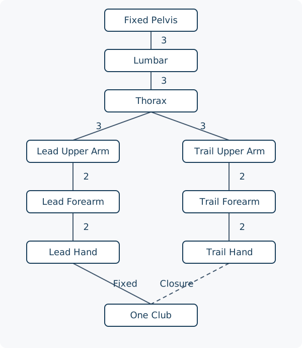{#fig-urdf_tree fig-alt="A fixed pelvis connects through lumbar and thorax joints to two arms. Each arm has shoulder, elbow and forearm, and wrist freedoms. One club attaches rigidly to the lead hand; a dashed trail-hand connection closes the loop."}
[]{#simplified-upper-body-model}
### A Reconciled Upper-Body Count
The nine bodies are pelvis, lumbar body, thorax, and three segments in each arm. Treat the fixed pelvis as the reference body: $N=9$. There are four three-DOF joints and four two-DOF joints. Their sum is 20 and their total nominal constraint count is $48-20=28$. Thus $6(9-1)-28=20$. Alternatively, introduce a separate ground body and one fixed pelvis-to-ground joint: both the extra body's six freedoms and the extra joint's six constraints cancel.
This count is for both arms, not for one arm plus both legs. A serial representation of the compound joints introduces virtual intermediate links. It changes the XML link and joint counts together without creating extra independent anatomical motion. Adding an independent pelvis yaw would add one freedom; changing to a fully floating pelvis would add six. Neither change is consistent with still calling the pelvis fixed.
[]{#the-grip-constraint-loop-closure}
### The Grip Constraint and the Club Body
[]{#princ-prin:dof_practice}
First rigidly attach the club to the lead hand. A rigid attachment adds a body and a fixed joint but no relative freedom. Requiring the trail-hand frame to match its prescribed grip frame on that club then adds a loop-closure condition. A full rigid relative pose supplies up to six independent scalar constraints. For a feasible configuration with closure rank six, the mobility becomes $20-6=14$.
The same result follows by initially making the club independent. A rigid club adds six freedoms once, giving $20+6=26$. Two rigid hand-to-club attachments nominally add twelve constraints. If their combined Jacobian has rank twelve, the result is $26-12=14$. These are alternative formulations of the same model; subtracting both counts in one formulation would count closure twice.
Finite-stiffness grips are different. Two compliant attachments exert forces and moments but do not each create a new independent club body. If both permit finite relative displacement, the rigid-segment configuration still has $20+6=26$ freedoms before any other exact constraints. Their force laws determine how those freedoms evolve. In a very stiff limit they may approximate rigid closure, but numerical stiffness, stored energy and contact reactions require separate analysis. Internal grip states or deformable shaft modes add further states only when explicitly modeled.
A point-coincidence grip supplies up to three constraints, a full rigid grip up to six, and a slipping or rolling contact has its own permitted directions. The rank of the combined Jacobian decides the count. Neither the word "grip" nor the number of hands specifies a unique constraint model.
[]{#freezing-vs.-freeing-dof}
### Adding Legs and Ground Contact
For each leg choose hip (3), knee (1) and ankle (2): six freedoms. Adding both legs to our fixed-pelvis upper-body tree gives $20+12=32$ internal freedoms. Releasing the pelvis to float gives 38. An earlier, different reduction using pelvis orientation (3), one spine joint (3), two legs (12) and two arms (14) also sums to 32; equal arithmetic totals do not make these the same model.
For illustration, give the floating 38-DOF body one independent rigid club, then impose two rigid feet and two rigid grips. If the combined 24 closure rows are independent and geometrically compatible, mobility is $38+6-24=20$. This is a local count for an ideal contact mode. It says nothing about whether the required ground wrenches lie inside friction and support limits, whether a foot should lift, or whether the golfer can supply the required joint torque.
Stack foot and hand constraints before evaluating their rank. When a heel rises or a foot slips, the contact mode and constraint matrix change. Position continuity alone does not settle velocity jumps at impact. A fixed-pelvis upper-body simulation, a floating-body simulation with ground contact, and a prescribed-pelvis simulation answer different questions about how ground interaction influences the club.
[]{#the-human-arm-----a-7-dof-redundant-manipulator}
[]{#the-human-arm-a-7-dof-redundant-manipulator}
## The Human Arm --- A Seven-DOF Redundant Manipulator
[]{#sec-arm_redundancy}
[]{#dof-counting-in-practice}
[]{#dof-count}
[]{#dof-count-and-redundancy}
### DOF Count and the Selected Task
The seven-DOF arm is useful because it separates joint motion from a hand task. A hand position lies in $\mathbb R^3$. A full rigid hand pose lies in $SE(3)$, a six-dimensional manifold, rather than globally in a single $\mathbb R^6$ coordinate chart. Locally one can differentiate task coordinates or use an appropriate spatial/body twist, keeping the frame and angular/linear ordering consistent.
For a seven-DOF arm with a feasible, regular full-pose task of rank six, the instantaneous task-null space has dimension one. For a regular position-only task of rank three it has dimension four. These dimensions assume the shoulder base is fixed and no additional loop or anatomical constraints remove motion. A singular or mechanically restricted arm can have a lower task rank.
More detailed anatomy changes the chosen configuration. For example, @Holzbaur2005 include 15 freedoms spanning shoulder, elbow, forearm, wrist, thumb and index finger, together with 50 muscle compartments. That model is evidence of an explicit modeling choice, not justification for assigning a universal number of freedoms to every golfer or every coaching description.
[]{#null-space-of-the-jacobian}
[]{#intuition-the-elbow-circle}
[]{#null-space-optimization-elbow-swivel}
### The Null-Space Motion: Elbow Swivel
[]{#ex-elbow_swivel}
Hold the shoulder center $S$ and wrist center $W$ fixed. Idealize upper arm and forearm as rigid segments with lengths $a$ and $b$. Let $D=\|W-S\|$, with $|a-b|<D<a+b$. The elbow center $P$ satisfies $\|P-S\|=a$ and $\|P-W\|=b$. The two spheres intersect in a circle. With $e=(W-S)/D$ and orthonormal $e_1,e_2$ perpendicular to $e$, define
$$
\begin{aligned}
c&=\frac{a^2-b^2+D^2}{2D},& r&=\sqrt{a^2-c^2},\\
P(\psi)&=S+ce+r(e_1\cos\psi+e_2\sin\psi).
\end{aligned}
$$
This describes a workspace circle of possible elbow centers, not necessarily a globally closed curve in joint coordinates. If elbow flexion $\beta=0$ denotes a straight arm, the cosine law gives $\cos\beta=(D^2-a^2-b^2)/(2ab)$. Fixed shoulder-to-wrist distance fixes the flexion angle in this ideal geometry. Swivel therefore requires coordinated rotations; it is not isolated elbow flexion.
Holding hand orientation as well as wrist position requires the shoulder, forearm and wrist rotations to compensate compatibly. Anatomical limits and collisions can truncate the circle to arcs or disconnected feasible pieces. At a straight or fully folded limit the circle degenerates. If $D=0$ and $a=b$, the above formula is undefined and the sphere-intersection geometry is different. These exceptions are part of the model, not small numerical inconveniences.
### Why Redundancy Matters for Golf
At a particular club pose, different feasible internal configurations can give different mass matrices, moment arms, joint loads, collision clearances and future reachable motions. This is a mechanical reason to study internal configuration rather than judging a swing only by the club's appearance. It does not establish that every configuration is equally useful or that every golfer can realize it.
Two arms gripping the same club cannot generally swivel independently while holding the torso and both grip frames fixed. The combined closure and task Jacobians decide which coordinated variations remain. If a model predicts alternatives, their dynamic feasibility must still be tested with torque, contact, activation and speed constraints over the relevant time interval.
[]{#the-elbow-circle-----a-concrete-null-space-motion}
[]{#the-pseudoinverse-solution-and-null-space-projection}
### The Pseudoinverse and Null-Space Projection
In local joint coordinates let $\dot y=J\dot q$. For a wide, full-row-rank $J$, its Euclidean Moore--Penrose inverse is $J^+=J^T(JJ^T)^{-1}$. The expression $(J^TJ)^{-1}J^T$ instead requires full column rank and is invalid for this redundant case. In general use an SVD, with an explicit tolerance and physically meaningful coordinate scaling.
If $\dot y_d$ lies in the range of $J$, every exact velocity solution has the form
$$
\dot q=J^+\dot y_d+(I-J^+J)w.
$$
[]{#eq-ch23_pseudoinverse_solution}
Here $w$ has joint-velocity units. The first term has minimum Euclidean norm in the chosen coordinates, not automatically minimum energy, muscle activation or joint load. If the target is outside the range, $JJ^+\dot y_d$ is a projection and the remaining task residual is nonzero. A damped inverse bounds amplification near rank loss by accepting task error; its nominal "null" projector generally leaks into the task.
[]{#summary-the-manifold-of-solutions}
## Kinematic Redundancy and the Manifold of Solutions
[]{#laymans-box:ch23_redundancy_intro}
[]{#sec-manifold_solutions}
[]{#redundancy}
### The Redundancy Problem
Let $\mathcal Q_c$ be the admissible configuration manifold after exact closures and let $F$ map it to the declared task:
$$
F:\mathcal Q_c\longrightarrow\mathcal Y,\qquad y=F(q).
$$
[]{#eq-ch23_task_space}
For club pose, $\mathcal Y=SE(3)$; for a selected point's position, $\mathcal Y=\mathbb R^3$. A speed objective, impact event or target ball flight adds further structure. In particular, "square face with maximum speed" is not fully specified by the six club-pose coordinates. Speed belongs to velocity state and an optimization objective; impact also depends on time and collision conditions.
With $\dim\mathcal Q_c=d$ and task differential rank $r$ at a regular point, local redundancy is
$$
d_{\mathrm{null}}=d-r.
$$
[]{#eq-ch23_redundancy_dof}
Thus the fixed-pelvis, rigid-two-grip upper-body model has $d=14$ under our rank assumptions. A further regular six-dimensional club-pose task would leave eight local configuration directions. Using the original open-tree count $20-6=14$ for that same closed model would omit the grip closure.
[]{#the-task-jacobian-and-the-null-space}
### The Task Jacobian on Admissible Velocities
[]{#def-ch23_null_space}
Choose a full-column-rank basis $Z(q)$ for $\ker A(q)$, so every admissible velocity can be written $v=Z\nu$. The task velocity is
$$
\dot y=J(q)v=J(q)Z(q)\nu.
$$
[]{#eq-ch23_task_jacobian}
The relevant rank is that of $JZ$, not the unconstrained $J$. The physical task-null velocities satisfy both conditions:
$$
\mathcal N_q=\{v:A(q)v=0,\ J(q)v=0\}.
$$
[]{#eq-ch23_null_space_def}
Equivalently their dimension is $n_v-\operatorname{rank}[A^T\ J^T]^T$. The choice of basis $Z$ changes the numerical representation but not this physical subspace. Choosing a metric is additional: it determines what counts as a small velocity, a costly torque or a statistically large deviation.
[]{#dimension-of-the-solution-manifold}
### The Solution Manifold
For a prescribed attainable target $y_0$, define the level set
$$
\mathcal S(y_0)=\{q\in\mathcal Q_c:F(q)=y_0\}.
$$
[]{#eq-ch23_solution_manifold}
If $F$ has constant rank $r$ in a neighborhood of the point, the constant-rank theorem gives a local level-set manifold of dimension $d-r$.
[]{#thm-ch23_manifold_dimension}
This is a local statement. It neither proves the target is reachable nor makes disconnected inverse-kinematics branches one smooth global surface. Joint limits add boundaries and corners; singular points need separate treatment.
An instantaneous null vector preserves the task to first order. For a finite step $q+\epsilon v$, the second-order term in the Taylor expansion can change $F$. To maintain the task during finite motion, update the null space as the configuration changes and solve or stabilize closure throughout the integration. The curvature of the level set explains why a straight step tangent to it can leave it.
### Different Golfers, Different Paths
[]{#princ-prin:ch23_motor_equivalence}
Equal impact pose does not imply equal impact velocity, equal timing or equal trajectories. Even equal pose and velocity of a chosen club frame do not by themselves establish equal ball flight without matching strike location, ball state, surface interaction and the collision model. Conversely, matching a complete club trajectory can still leave internal motion unobserved.
The existence of this redundancy is a mathematical property of the chosen map. Showing that golfers organize variability along it requires data. @Myers2008 measured torso/pelvis kinematics and ball velocity in 100 recreational golfers; those associations do not establish equality of club trajectories or identify null-space torques. @Glazier2011 discuss competing interpretations and methods for movement variability. Neither source supplies a universal count of freedoms "used" by novices and experts.
### Bernstein's Degrees of Freedom Problem
[]{#laymans-box:ch23_freezing_freeing}
[]{#def-ch23_bernstein_problem}
The coordination question is how an organism produces reliable task behavior with many available internal variables. A mathematical redundancy creates room for coordination; it does not identify the nervous system's algorithm. Reduced variation in some joint angles can reflect a chosen strategy, physical limits, an imposed task, measurement noise, or correlations among coordinates.
Likewise, the number of principal components explaining a dataset's variance is not the number of anatomical freedoms. It depends on normalization, sampled movements, noise and the retained variance threshold. A learned low-dimensional controller can command a mechanism whose configuration remains high-dimensional. Any claim that skill "releases" a particular number of freedoms must define and measure that number rather than substitute a suggestive metaphor.
[]{#self-organization-through-constraints}
[]{#compensation-patterns}
### Self-Organization, Compensation and Evidence
Constraints and feedback can organize coordinated motion without a controller explicitly solving every equation in this chapter. Optimization is one candidate description, alongside other control models. Its success in a simulation is a prediction under assumed dynamics, information and costs, not direct evidence that the brain computes that optimization.
Restricted motion in one joint can change the feasible set and the effort needed elsewhere. Whether an alternative movement preserves a particular golf outcome is an empirical question involving the individual, task and available control. Kinematic redundancy alone does not establish that compensation succeeds, reduces tissue load or prevents injury. A useful technical account reports the predicted alternatives and the measurements that could distinguish them.
[]{#the-7-dof-arm-----redundancy-in-miniature}
[]{#the-7-dof-arm-redundancy-in-miniature}
## The Seven-DOF Arm --- Redundancy in Miniature
[]{#sec-arm_redundancy_detailed}
[]{#the-elbow-circle-a-concrete-null-space-motion}
### A Concrete Elbow-Circle Calculation
Take $a=0.30$ m, $b=0.25$ m and $D=0.40$ m. The circle center lies $c=0.234375$ m from the shoulder along the shoulder-to-wrist axis and its radius is approximately $0.18727$ m. Sampling the circle preserves both segment lengths; the elbow flexion is constant because $\cos\beta=0.05$. The wrist orientation still requires compatible compensating rotations. These are dimensions of a teaching geometry, not a participant's measurements.
Adding a prescribed elbow height can remove one additional local degree of redundancy if its differential is independent on the remaining level set. For a full-pose, rank-six arm, that can leave isolated solutions locally. It need not select a unique global configuration: a horizontal plane can intersect the elbow circle at two points. At a tangent intersection or when the entire circle has that height, the rank argument changes. With a position-only task, the four-dimensional task-null space is not exhausted by describing one elbow circle.
[]{#elbow-swivel-in-the-golf-swing}
[]{#a-simplified-golf-swing-urdf-upper-body}
### Application to the Golf Swing
Suppose two feasible address configurations place both grips and the club identically. Their future behavior under the same torque history need not match: inertia and drift depend on configuration, and contact reactions may differ. If one configuration permits a better future speed/accuracy tradeoff, the reason must be demonstrated through the dynamics and the stated objective.
This also clarifies a common verbal mistake. Once a particular club velocity is prescribed, a task-null velocity cannot increase that same velocity at that instant. It can change posture while preserving the prescribed velocity, and that posture may affect subsequent acceleration or feasible control. "Preserve the present task while improving a future option" is a precise claim that can be investigated.
## Redundancy and Null-Space Control
[]{#dc-box:ch23_null_space_ztcf}
[]{#sec-null_space_control}
[]{#from-anatomy-to-equations}
### From Joint Velocities to Applied Torques
For the moment use unconstrained local coordinates with $v=\dot q$, symmetric positive-definite mass matrix $M(q)$ and generalized dynamics
$$
M(q)\dot v+h(q,v)=B(q)u.
$$
$h$ collects the specified inertial, gravitational and passive terms on the left. $B$ maps the chosen inputs into generalized forces. With independent joint torques, $B=I$. With muscle forces, $B$ contains moment-arm information; with neural commands, activation dynamics may prevent the command from acting directly in this acceleration equation.
For $x=(q,v)$ the torque-driven state equation is
$$
\dot x=f(x)+G(x)u,\qquad
G=\begin{bmatrix}0\\M^{-1}B\end{bmatrix}.
$$
[]{#eq-ch23_ztcf_system}
If $B=I$, $G$ is injective: no nonzero joint torque disappears from the full-state derivative. Task redundancy therefore does not imply a nontrivial kernel of the full-state actuation map. A zero-torque counterfactual also retains the terms assigned to $h$ and any retained activation or elastic states according to its declared intervention. Removing the specified torque commands is not synonymous with removing every biological or stored-energy contribution.
### The Acceleration-Level Task Map
Differentiating $\dot y=Jv$ gives
$$
\ddot y=JM^{-1}Bu-JM^{-1}h+\dot Jv.
$$
At the same configuration and velocity, changing the input by $\delta u$ changes task acceleration by $JM^{-1}B\delta u$. The input-null condition is therefore $JM^{-1}B\delta u=0$. It differs from the velocity-null condition $J\delta v=0$. Dropping $\dot Jv$ or gravity would also produce an incorrect absolute acceleration even if the input difference were computed correctly.
For an elementary counterexample, take $M=\operatorname{diag}(2,1)$ and $J=[1\ 1]$ in consistent chosen units. The velocity $(1,-1)^T$ lies in $\ker J$. Applying the same components as a generalized torque gives $JM^{-1}(1,-1)^T=-1/2$, so the task accelerates. This calculation isolates the mass-matrix distinction without appealing to a complicated human simulation.
[]{#pedagogical-simplification}
[]{#automatic-dynamics-computation}
### A Dynamically Consistent Projection
When $J$ has full row rank, define
$$
\begin{aligned}
\Lambda&=(JM^{-1}J^T)^{-1},\\
\bar J&=M^{-1}J^T\Lambda,\qquad N=I-\bar J J.
\end{aligned}
$$
Then $J\bar J=I$ and $JN=0$. The velocity $\bar J\dot y$ minimizes instantaneous kinetic energy among velocities realizing $\dot y$, under this unconstrained model. The corresponding torque decomposition uses the transpose projector:
$$
\tau=J^TF+N^T\tau_0,\qquad JM^{-1}N^T=0.
$$
[]{#eq-ch23_control_decomposition}
Indeed $JM^{-1}N^T=JM^{-1}-JM^{-1}J^T\bar J^T=0$ because $\bar J^T=\Lambda JM^{-1}$. This is instantaneous dynamic consistency, as developed in [Khatib's operational-space analysis](https://khatib.stanford.edu/publications/pdfs/Khatib_1990_2.pdf). $F$ still must account for drift and the desired task acceleration. A projection does not automatically construct the complete tracking controller.
For the numerical example above, $\bar J=(1/3,2/3)^T$. $N$ maps velocities into $\ker J$, while $N^T$ maps torques into $\ker(JM^{-1})$. Interchanging them would erase the distinction the derivation was meant to capture. Neither null torque nor null velocity implies zero internal energy change. Power remains $\tau^Tv$, and a null input can alter subsequent state, limits and task sensitivity.
### Contact, Underactuation and Internal Grip Forces
For stationary ideal constraints use
$$
M\dot v+h=Bu+A^T\lambda,\qquad A\dot v+\dot A v=0.
$$
Assume $A$ has independent rows. Eliminating the constraint reaction gives
$$
\begin{aligned}
K&=AM^{-1}A^T,\\
W&=M^{-1}-M^{-1}A^TK^{-1}AM^{-1},\\
\dot v&=W(Bu-h)-M^{-1}A^TK^{-1}\dot A v.
\end{aligned}
$$
Here $AW=0$: $W$ maps generalized force changes into admissible acceleration changes. The task input map becomes $JWB$. Redundant constraints require removing dependent rows or a justified generalized inverse; unilateral/frictional contact also requires checking whether the assumed mode remains valid. A floating body generally lacks direct actuation of its base coordinates. Consequently an arbitrary generalized null torque need not be implementable by its joint actuators.
Inputs that leave all admissible accelerations unchanged may nevertheless change constraint reactions. With two hands, opposing forces can cancel in the net club wrench while changing the loads at each grip. This force redundancy is not the same as an elbow-swivel velocity. The [multicontact analysis of Sentis, Park and Khatib](https://cs.stanford.edu/groups/manips/publications/pdfs/Sentis_2010_TRO.pdf) connects support constraints, task control and internal forces under explicit actuation/contact assumptions. It does not provide evidence for a particular golfer's neural strategy.
Ideal stationary constraints do no net work on admissible motion because $(A^T\lambda)^Tv=\lambda^TAv=0$. Individual bodies can exchange power through their common constraint forces. Compliant grips can store or dissipate energy, and prescribed moving constraints can supply power. Distinguishing system boundary and constraint law is necessary before interpreting an internal force as an energy source.
[]{#null-space-optimization-in-the-ztcf-family}
### Null-Space Optimization and Its Limits
[]{#ex-ch23_elbow_swivel_null_space}
For an unconstrained kinematic task with an Euclidean projector $P=I-J^+J$, one can choose $w=-k\nabla H(q)$ to favor a posture cost $H$, with $k>0$. The null contribution to $\dot H$ is $-k\nabla H^TP\nabla H\leq0$. The task-producing term $J^+\dot y_d$ can still increase $H$, so the full cost need not decrease. Joint limits, non-Euclidean metrics and closed loops require the corresponding constrained formulation.
A torque-level objective requires the acceleration dynamics, not substitution of the same $w$ into a torque port. Force limits, muscle activation dynamics, grip feasibility and future tasks can defeat a locally attractive direction. For golf, a credible optimization specifies the horizon, impact event, observations, controls and tradeoff between speed and accuracy; then reports feasibility and sensitivity, not only the optimizer's preferred posture.
[]{#grübler-kutzbach-formula}
## URDF --- The Unified Robot Description Format
[]{#sec-urdf}
[]{#basic-structure}
[]{#key-urdf-tags}
[]{#kinematic-structure}
### Basic Structure and Frames
URDF describes a tree of links connected by joints. Every non-root link has one parent joint; the root has none. Each joint specifies a parent, child, origin transform and joint type. A conventional revolute joint axis is expressed in its joint frame. The zero-position transform and rotation sequence are part of the definition: changing them while retaining the same angle values changes the physical pose. Consult the [URDF model API](https://docs.ros.org/kinetic/api/urdf/html/index.html) for the underlying tree and joint representation, and the selected importer's documentation for supported features.
A root link called "world", "ground" or "pelvis" does not, by its name, specify every simulator's base behavior. A parser may fix it or add a floating joint according to its conventions and setup. Verify the imported joint types, $n_q$, $n_v$ and world attachment. Likewise, a displayed mesh is not evidence that the inertia or collision model matches it.
[]{#a-simple-example-2-link-arm}
### A Complete Two-Link Example
[]{#ex-urdf_simple}
The following complete tree has a base and two uniform solid cylinders of lengths $(0.30,0.25)$ m, masses $(2,1)$ kg and radius $0.02$ m. Their long axes are local $x$; the joints rotate about local $z$. Their COMs lie halfway along each cylinder. URDF cylinders are aligned with their geometry-frame $z$ axis, so the visual and collision frames are rotated by $\pi/2$ about $y$. The inertial frames remain aligned with the link frames, with the small longitudinal moment in the $xx$ entry.
Continuous joints are used for this unrestricted teaching mechanism. These are not physiological range-of-motion or torque-limit claims. Gravity, actuation and the time integrator are configured by the simulator separately.
```xml
<robot name="teaching_arm">
  <link name="base" />
  <link name="link1">
    <inertial>
      <origin xyz="0.15 0 0" rpy="0 0 0" />
      <mass value="2" />
      <inertia ixx="0.0004" iyy="0.0152" izz="0.0152" ixy="0" ixz="0" iyz="0" />
    </inertial>
    <visual>
      <origin xyz="0.15 0 0" rpy="0 1.57079632679 0" />
      <geometry>
        <cylinder radius="0.02" length="0.3" />
      </geometry>
    </visual>
    <collision>
      <origin xyz="0.15 0 0" rpy="0 1.57079632679 0" />
      <geometry>
        <cylinder radius="0.02" length="0.3" />
      </geometry>
    </collision>
  </link>
  <joint name="joint1" type="continuous">
    <parent link="base" />
    <child link="link1" />
    <origin xyz="0 0 0" rpy="0 0 0" />
    <axis xyz="0 0 1" />
  </joint>
  <link name="link2">
    <inertial>
      <origin xyz="0.125 0 0" rpy="0 0 0" />
      <mass value="1" />
      <inertia ixx="0.0002" iyy="0.00530833333333" izz="0.00530833333333" ixy="0" ixz="0" iyz="0" />
    </inertial>
    <visual>
      <origin xyz="0.125 0 0" rpy="0 1.57079632679 0" />
      <geometry>
        <cylinder radius="0.02" length="0.25" />
      </geometry>
    </visual>
    <collision>
      <origin xyz="0.125 0 0" rpy="0 1.57079632679 0" />
      <geometry>
        <cylinder radius="0.02" length="0.25" />
      </geometry>
    </collision>
  </link>
  <joint name="joint2" type="continuous">
    <parent link="link1" />
    <child link="link2" />
    <origin xyz="0.3 0 0" rpy="0 0 0" />
    <axis xyz="0 0 1" />
  </joint>
</robot>
```
The downloadable [teaching_arm.urdf](../models/teaching_arm.urdf) and the generator `TwoLinkArm.urdf()` use the same model. A content test checks that they agree. This example is a verifiable building block; the open two-link tree does not implement a golfer's two-hand closure, foot contacts or muscle physiology.
[]{#urdf-joint-types}
### Link Inertia and Joint Semantics
[]{#def-urdf_link}
[]{#def-urdf_joint}
An inertial origin specifies the COM position and the orientation of the inertia frame relative to the link. The six independent inertia entries describe the symmetric rotational inertia about that COM in that frame, in kg m$^2$. They must not be copied from a tensor about a joint origin without a parallel-axis correction. For a uniform cylinder along $x$,
$$
I_{xx}=\frac12 mr^2,\qquad I_{yy}=I_{zz}=\frac{m}{12}(3r^2+L^2).
$$
The first cylinder has moments $(0.0004,0.0152,0.0152)$ kg m$^2$. For the second cylinder they are approximately $(0.0002,0.00530833,0.00530833)$ kg m$^2$. Positive mass and symmetric positive-definite rotational inertia are necessary for nondegenerate solid bodies. Principal moments must also obey the triangle inequalities, such as $I_1+I_2\geq I_3$; positive eigenvalues alone do not establish physical realizability.
If $R$ expresses the inertia frame in another frame, rotate the tensor as $R I_C R^T$. To move its reference point by displacement $d$ from COM to the new origin, add $m(\|d\|^2I-dd^T)$. Rotation and translation perform different operations. Summing segment tensors requires expressing them about the same point and in the same frame.
### Compound Joints and Closed Loops
Standard revolute, continuous, prismatic and fixed joints represent their specified relative motions. Floating and planar joint support varies by importer. A three-axis shoulder represented by serial ZYX revolutes needs two intermediate virtual links between the physical parent and child. The axes are successive local axes, and the Euler-angle rate map becomes singular at its chart's gimbal-lock orientations. An ideal spherical joint has three physical rotational freedoms without that particular chart singularity.
Virtual links represent coordinate frames, not new pieces of anatomical tissue. A dynamics engine may reject massless moving links or treat them specially. Adding small masses to make a parser accept them changes inertia; it requires an explicit regularization study. Where supported, native multi-DOF joints or multiple joint primitives on one physical body can avoid this artificial mass assignment.
The URDF tree cannot give a child link two parents. Choose a spanning tree and add the omitted rigid closure through the engine's constraint mechanism, or define a compliant attachment with stated force and energy laws. Do not duplicate the club as two independent bodies, silently weld away intended motion, or expect a second parent tag to create a valid two-hand model.
[]{#building-a-full-body-golf-urdf}
## Building a Full-Body Golf Model
[]{#sec-golf_urdf}
[]{#segment-parameters-anthropometry}
### A Construction Sequence That Preserves the Physics
Begin with the nine-body, eight-compound-joint upper-body blueprint and document every physical segment and reference frame. Decide whether the pelvis is fixed, prescribed or floating before adding ground contact. Add legs only when the research question needs their motion and reaction forces; add a head or detailed hands when their inertia or task role matters. Assign the club once, with measured or explicitly idealized mass, COM and inertia.
Then choose the joint representation, including pronation and shoulder-girdle approximation, and verify forward kinematics at recognizable poses. Add one grip to the spanning tree and the second as an explicit closure, or use two compliant attachments. At a feasible reference pose compute the constraint rank and residual. Finally add actuators and their states, contact parameters and the controller. Each addition should have a mechanical check before interpreting a full swing.
Calling this a musculoskeletal model requires more than a file of rigid links. Muscle paths, moment arms, force--length and force--velocity behavior, activation dynamics and any tendon compliance must be defined when those mechanisms support the argument. A tendon path in a simulator is not by itself a muscle activation model. Parameter provenance and validation must match the scientific claim being made.
[]{#anthropometric-data-de-leva-1996}
### Anthropometry: Segment Definitions Come First
[]{#ex-anthropometry}
@DeLeva1996 adjusted segment parameters derived from Zatsiorsky--Seluyanov's gamma-scanning measurements of living subjects, using additional anthropometric information to change reference landmarks. This was not a new cadaver-measurement study. Population estimates provide a starting model, not an individual's measured inertia. Using their values requires matching the segment boundaries, sex-specific table, COM endpoints and inertia-axis definitions.
For orientation, selected male segment mass fractions from Table 4 are: upper arm $2.71%$, forearm $1.62%$, hand $0.61%$, thigh $14.16%$, shank $4.33%$ and foot $1.37%$ of body mass, each for one segment. The whole-trunk value is $43.46%$. A table containing whole trunk plus its subparts would double-count mass. Nor can a generic "thorax" fraction and an undefined "lumbar" body be assigned independently and presumed to preserve the original partition.
The same table gives the male forearm longitudinal radius of gyration as $12.1%$ of the specified segment length. That yields $I_{\mathrm{long}}=m(0.121L)^2=0.014641mL^2$, not $0.121mL^2$. Alternative endpoint definitions change the normalized coefficient. The published URDF example uses derived cylinder inertias instead, so its geometry and mass properties can be checked without presenting population means as subject anatomy.
[]{#pinocchio-inria}
[]{#looking-ahead}
### Scaling Mass, Length and Inertia
For an unchanged segment definition, scaling body mass from 70 to 80 kg while retaining mass fractions multiplies segment masses by $80/70$. If every segment's geometry is unchanged and only density changes uniformly, its inertia scales by the same factor. If lengths also scale by $s_L$ with geometrical similarity, inertia scales by $s_m s_L^2$ and COM distances by $s_L$. With unchanged density, $s_m=s_L^3$, giving inertia scaling $s_L^5$.
These are conditional scaling laws, not proof that two people have similar segment shapes or densities. If a lumbar segment is repartitioned, its mass, COM and inertia must be recomputed together. A subject-specific optimization must maintain physical consistency while fitting measurements; independently perturbing all tensor entries can generate nonphysical bodies even when each entered number looks plausible.
## From URDF to Simulation --- Drake, MuJoCo and Pinocchio
[]{#sec-simulation_engines}
### What the Software Supplies
**Drake** provides multibody modeling within a systems and optimization framework. Its [Parser](https://drake.mit.edu/pydrake/pydrake.multibody.parsing.html) adds model instances to a plant; the returned model-instance identifiers are not the plant itself. A usable setup creates the plant, parses into it, specifies world attachment and actuation as needed, finalizes the plant, creates a context and supplies state/input before simulation. This distinction matters when translating a short API sketch into an executable experiment.
**MuJoCo** compiles URDF or its native MJCF into a model and advances a separate data/state object. MJCF exposes richer engine-specific constraints, tendons and actuators. Its [modeling documentation](https://mujoco.readthedocs.io/en/3.4.0/modeling.html) allows multiple primitive joints on one physical body, avoiding dummy bodies for such compound representations. An RL algorithm remains a separate controller/training procedure; a physics engine does not itself establish policy learning or biological validity.
**Pinocchio** supplies rigid-body algorithms including inverse dynamics, generalized inertia, kinematics and Jacobians, with URDF parsing, as described in its [official feature documentation](https://stack-of-tasks.github.io/pinocchio/). A dynamics library, numerical integrator, contact solver, derivative evaluator and trajectory optimizer are distinct components even when a larger package integrates them. Select and test the required combination rather than ranking software by an unsupported steps-per-second number.
### An Executed Import and Dynamics Check
[]{#ex-auto_dynamics}
Run the following from the repository root with Python 3.12, NumPy and MuJoCo 3.4.0. The version is stated because signatures can change; the installed version's `mj_fullM` accepts the model, destination dense matrix and sparse inertia array in that order. The XML path is relative to the repository, and the checked root interpretation is fixed. No GUI or training run is required.
```python
import mujoco
import numpy as np

model = mujoco.MjModel.from_xml_path(
    "articles/The_Physics_of_Golf/models/teaching_arm.urdf"
)
model.opt.gravity[:] = [0, -9.81, 0]
model.opt.timestep = 0.0005
model.opt.integrator = mujoco.mjtIntegrator.mjINT_RK4
data = mujoco.MjData(model)
data.qpos[:] = [0.3, 0.7]
mujoco.mj_forward(model, data)
mass = np.empty((model.nv, model.nv))
mujoco.mj_fullM(model, mass, data.qM)
print(model.nq, model.nv, model.nu)
print(mass, data.qfrc_bias.copy())
data.qfrc_applied[:] = [1.0, 0.0]
mujoco.mj_forward(model, data)
print(data.qacc.copy())
mujoco.mj_step(model, data, nstep=200)
print(data.time, data.qpos.copy(), data.qvel.copy())
```
The imported dimensions are $n_q=n_v=2$ and $n_u=0$: the URDF defines no actuator. Here `qfrc_applied` supplies external generalized torques directly, which is useful for a mechanics check but does not model bounded biological actuation. At $q=(0.3,0.7)$ rad and zero velocity, the independent and imported results agree:
$$
M\simeq\begin{bmatrix}0.22849650&0.04961492\\0.04961492&0.02093333\end{bmatrix},\qquad
h\simeq\begin{bmatrix}6.28565628\\0.66254570\end{bmatrix}.
$$
The units are kg m$^2$ for $M$ and N m for $h$. Applying $(1,0)$ N m gives initial accelerations approximately $(-33.50095,47.75165)$ rad/s$^2$. The positive distal acceleration follows from dynamic coupling and gravity; it is not evidence of a distal actuator command. After 200 RK4 steps of 0.0005 s, this model reaches $q\simeq(0.135246,0.915810)$ rad. A numerical trajectory is a result for the specified example, not a verified golf prediction.
[]{#example:four_bar_loop}
[]{#many-ways-to-reach-the-cup}
### Independent Mechanics Behind the Check
Let $c_i=L_i/2$ and let $I_i$ be each cylinder's centroidal $zz$ moment. Expanding the Cartesian translational and rotational kinetic energies gives
$$
\begin{aligned}
M_{11}&=I_1+m_1c_1^2+I_2+m_2(L_1^2+c_2^2+2L_1c_2\cos q_2),\\
M_{12}&=M_{21}=I_2+m_2(c_2^2+L_1c_2\cos q_2),\\
M_{22}&=I_2+m_2c_2^2.
\end{aligned}
$$
With downward global $y$ gravity, potential is $V=g[(m_1c_1+m_2L_1)\sin q_1+m_2c_2\sin(q_1+q_2)]$ and the zero-velocity bias is $\nabla V$. At nonzero velocity the bias also contains velocity-dependent terms. The tests compare $v^TMv/2$ against independently assembled Cartesian kinetic energy and compare $\nabla V$ with finite differences before checking the importer. Agreement between two calls into the same engine would be a weaker verification.
## Sensitivity Analysis --- What Happens When Parameters Are Wrong?
[]{#sec-sensitivity}
[]{#urdf-link}
[]{#urdf-joint}
### Sources of Uncertainty
Relevant uncertainties include segment boundaries and inertias, marker-to-bone motion, joint axes, club properties, external wrenches, initial velocities, actuator parameters and the contact model. State-estimation filtering can correlate errors across time and across coordinates. Finite differences used to estimate acceleration can magnify noise. Sampling frequency alone does not specify motion-capture accuracy or identify the correct model structure.
Uncertainty statements need units and an evidential basis. An orientation error is measured in radians or degrees; an angular-velocity error in rad/s or degrees/s. A perturbation range is an assumed scenario unless it is calibrated to measurements. There is no model-independent percentage by which a forearm mass error changes club speed, and no universal ordering that makes kinematic measurement accuracy more important than inertia accuracy for every output.
### Fixed-Control and Feedback Sensitivities
For a smooth fixed-mode system $\dot x=f(x,u,p)$, differentiate with respect to a parameter vector $p$ along a specified input history. With $S=\partial x/\partial p$,
$$
\dot S=f_xS+f_p,\qquad S(0)=\frac{\partial x_0}{\partial p}.
$$
If the controller is $u=\pi(x,p)$, the corresponding terms become $(f_x+f_u\pi_x)S+f_p+f_u\pi_p$. Holding a torque history fixed, replaying recorded commands and reoptimizing the controller for each parameter are different experiments. Report which is performed. An optimizer's improved value after reoptimization does not measure the same sensitivity as a golfer receiving an unanticipated perturbation.
For a fixed terminal time and output $z=\psi(x(T),p)$, $dz/dp=\psi_xS(T)+\psi_p$. A differentiable impact-time definition $H(x(t_*),p,t_*)=0$ adds event-time sensitivity:
$$
\frac{dt_*}{dp}=-\frac{H_xS(t_*)+H_p}{H_xf(t_*)+H_t}.
$$
The denominator must be nonzero. Terminal output derivatives then include the time-shift term $\psi_x f\,dt_*/dp$ and any explicit time dependence of $\psi$. Grazing events, changing contact modes and discontinuous controllers may invalidate this smooth calculation and require event/reset analysis.
[]{#interpretation}
[]{#practical-implications}
### A Bounded Numerical Interpretation
[]{#ex-sensitivity}
If a stated model gives $\partial v_{\mathrm{club}}/\partial m_f=-0.05$ (m/s)/kg and the only perturbation is $\delta m_f=\pm0.2$ kg, the first-order speed change is $\mp0.01$ m/s. At 45 m/s this is about $0.0222%$ of the nominal speed. These are hypothetical supplied numbers, not a measured golf sensitivity. Other parameter and state errors can dominate or cancel this contribution.
For a covariance $\Sigma$ of a parameter/state error vector and local output sensitivity row $s$, the linearized variance is $s\Sigma s^T$. Correlations matter. For interval assumptions, propagate the stated admissible set rather than labeling the result a confidence interval. Check nonlinear effects by finite perturbations and numerical convergence; do not infer a probability distribution from a convenient percentage sweep.
[]{#sensitivity-to-anthropometry}
[]{#sensitivity-of-club-speed-to-forearm-mass}
[]{#sensitivity-to-initial-conditions}
### Sensitivity to Initial Conditions and Robustness
Initial-state perturbations obey the variational equation $\dot\Phi=f_x\Phi$ for the specified open-loop system, or the corresponding closed-loop Jacobian. Large finite-time amplification is not by itself evidence of chaos. Proving chaotic dynamics needs a more specific dynamical claim than observing that a small start error changes an impact result.
[]{#princ-prin:sensitivity_practical}
For a useful robustness assessment, define the output or conclusion, the feasible uncertainty set, the controller and the contact/event rules. Compare multiple time steps and derivative perturbation sizes. Include parameter correlations and physically realizable inertias. State which conclusions persist and which change. A successful arbitrary $\pm20%$ sweep establishes only the tested scenarios; it cannot certify robustness outside them or determine the best measurement investment without a sensitivity comparison.
[]{#key-takeaways-from-urdf-to-physics}
## Building Intuition: From URDF to Golf Physics
[]{#sec-intuition}
[]{#task-space}
### The Redundancy Principle
The key connection is now explicit. Constraints determine the motion the body can make; the task map determines which of those motions appear at the club; inertia and actuation determine how forces change those motions. An internal configuration can preserve the present club pose while changing future acceleration authority. Grip-force distribution can preserve a resultant club wrench while changing loads on the arms. Those are complementary mechanical possibilities, each with its own observable consequences.
Redundancy is therefore an opportunity to investigate alternative feasible solutions, not a guarantee of greater efficiency, safety or consistency. A model that omits a material wrist, grip or elastic state can hide a relevant pathway even if its joint-angle fit is excellent. A model that adds detail without identifiable parameters can create unwarranted confidence. The appropriate resolution is the one needed to answer and test a stated question.
### The Identification Problem
Club trajectory alone generally does not recover full-body joint motion. Full-body kinematics alone generally does not recover unknown external contact wrenches. If inertial parameters, full state/acceleration and all external loads are known, inverse dynamics determines the required net generalized force in the specified model. Splitting that net force among muscles remains another inverse problem, especially with multiple muscles and co-contraction.
Likewise, a fitted inverse-optimal-control cost is not uniquely the nervous system's objective. Multiplying a cost by a positive constant preserves its minimizers, and different costs can agree along one observed trajectory while disagreeing elsewhere. Model error, unmeasured constraints and assumed feedback information can all be absorbed into fitted weights. Cross-condition predictions and controlled perturbations are more informative than fitting one successful swing.
A strong study therefore states the forward model and which quantities are measured, reports parameter/state uncertainty and residuals, and tests predictions on conditions withheld from fitting. Depending on the question, discriminating data might include force-plate wrenches, grip loads, additional segment kinematics or activation-related measurements with their own observation model. No single sensor automatically closes every level of this inverse problem.
### What We Can Now Claim
[]{#princ-prin:ch23_summary}
We can count regular mobility for a declared model, compute task-null directions on its admissible velocity space, distinguish them from torque-null inputs, and verify a rigid-body file against mechanics. These tools make competing explanations concrete. They do not yet establish a unique control strategy, a complete musculoskeletal representation or a universal best swing.
The next step is to ask how control works with limited information, delay and noisy measurements. Those constraints belong alongside anatomy, mechanics and task geometry in an explanation of the golf swing. Preserving their distinctions makes their interaction more understandable, not less.
## Primary Sources and Reading Guidance
1. [Lynch and Park, Mobility](https://modernrobotics.northwestern.edu/nu-gm-book-resource/2-2-degrees-of-freedom-of-a-robot/), and [Singularities](https://modernrobotics.northwestern.edu/nu-gm-book-resource/5-3-singularities/): independent constraints, task Jacobians and rank; these are mechanisms lessons, not human motor-control measurements.
1. [Khatib, Dynamic Consistency](https://khatib.stanford.edu/publications/pdfs/Khatib_1990_2.pdf): operational-space inertia and torque projection. Follow the dimensions of every matrix when reading the scanned equations.
1. [Sentis, Park and Khatib (2010)](https://cs.stanford.edu/groups/manips/publications/pdfs/Sentis_2010_TRO.pdf): multicontact and internal-force control, under the paper's contact and actuation assumptions.
1. [de Leva (1996)](https://doi.org/10.1016/0021-9290(95)00178-6): adjusted segment definitions, Table 4 and reference endpoints. Do not combine whole-trunk and trunk-subsegment fractions.
1. [Holzbaur, Murray and Delp (2005)](https://pubmed.ncbi.nlm.nih.gov/16078622/): an explicit arm and hand model; compare retained joints and muscles before transferring its parameters.
1. [Myers and Colleagues (2008)](https://pubmed.ncbi.nlm.nih.gov/17852693/) and [Glazier (2011)](https://pubmed.ncbi.nlm.nih.gov/21699094/): torso/pelvis associations and the interpretation of movement variability, respectively; neither identifies the torque-null controller of a golfer.
1. [MuJoCo 3.4 Python Bindings](https://mujoco.readthedocs.io/en/3.4.0/python.html), the linked modeling manual, URDF API, Drake Parser and Pinocchio feature documentation: verify importer semantics and runtime version independently of scientific validation.
::: {.callout-note}
## On This Site
- **[Model Ladder](../../../models/model-ladder.html)** — Progressive model complexity for human and equipment systems
- **[Degrees of Freedom and Dimensionality](../../degrees-of-freedom-and-dimensionality.html)** — State dimension, observability, and control authority
:::
## Chapter Exercises
[]{#exercises-ex:ch23_exercises}
1. **DOF Counting:** Reconstruct the nine-body upper-body model's 20 freedoms using both joint summation and the spatial constraint count. Add the club first as a rigid lead-hand attachment and then as an independent body. Under full-rank rigid-grip closure, obtain 14 in both formulations. Repeat with two compliant grips, then explain why nominal foot constraints must be stacked with grip constraints before making a full-body count.
1. **Null-Space Motion:** For the regular seven-DOF arm distinguish a rank-three position task from a rank-six pose task. Derive the elbow circle for fixed shoulder/wrist centers and prove flexion is constant. Add a prescribed elbow height, stating the independence assumption and the possible global multiplicity. Explain why one circle does not parameterize all four freedoms of the position-only null space.
1. **URDF Construction:** Starting from the complete two-link file, verify every COM, cylinder orientation and principal inertia. Design a kinematic spine/arm tree with two three-axis compound joints. Count the intermediate virtual links needed for six serial revolutes and identify the reference body. Describe the selected engine's treatment of massless frames or native multi-DOF joints before claiming a valid dynamic model; do not assign undocumented artificial tissue mass.
1. **Anthropometric Scaling:** Scale a 70 kg model to 80 kg with unchanged segment geometry, then repeat with an independent uniform length factor $s_L$. Derive the inertia factors in both cases and under fixed-density geometrical similarity. Explain why changing trunk partitions requires recomputing COM and inertia, not only multiplying masses.
1. **Sensitivity Calculation:** Use the hypothetical derivative $-0.05$ (m/s)/kg with mass perturbation $\pm0.2$ kg to calculate the local speed change and its fraction of 45 m/s. State what additional evidence is needed to call this a confidence interval. Derive how a differentiable impact-time condition modifies the output derivative and identify the grazing-event failure condition.
1. **Loop Constraints and Forces:** Contrast a point grip, rigid grip and compliant grip. For $M=\operatorname{diag}(2,1)$ and $J=[1\ 1]$, show that $(1,-1)^T$ is velocity-null but not torque-null. Construct $\bar J$, $N$ and $N^T$ and verify their respective identities. Explain how two opposing grip forces can alter hand loads without altering the net club wrench.
1. **Redundancy in Golf:** Formulate two dynamically feasible candidate swings that agree in a declared club task but differ internally. Specify whether the agreement is at one impact pose, impact state or the entire trajectory. Identify an observable that could distinguish the candidates and a perturbation that tests their predicted future behavior. Explain why a fitted trajectory alone does not identify the brain's unique objective or prove reduced injury risk.
